
By Paul Mahon, iFormulate Associate Partner, November 2014
 Most of the science needed to predict, control and define the stability of solutions was defined by scientists of the Victorian era such as Ostwald and Arrhenius. Nevertheless, as formulation chemists, we still regularly encounter poor stability in liquid solution products. The reason for this, I believe, is that solubility and stability studies are still sometimes regarded as trivial and so are not properly thought out and executed.
So how do we ensure that our solutions remain stable? Firstly, we need to measure the true solubility of our solutes, then we need to assess the physical and chemical stability of any solutions we make with them.
The solubility of a material is the concentration of the solute in a steady state, saturated solution at any given temperature. The solubility of a solid generally increases with increasing temperature and is often (but not always) greater when the melting point is lower and the latent heat of melting is smaller.
In practice real-world solubility measurements are not usually absolute and many things can influence the apparent solubility, important factors are:
1. Supersaturation: Simply dissolving a solute in solvent, especially if you use agitation, heat or ultrasound will usually create an thermodynamically unstable “supersaturated” solution.
2. Purity: generally speaking the purer the (solute) material is then the lower its solubility will be.
3. Measurement method: The apparent solubility can sometimes vary depending on how you measure it.
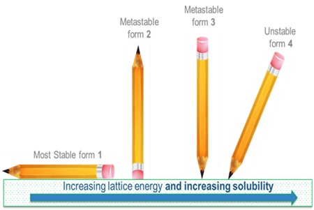
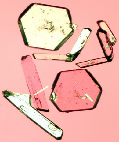 4. Polymorphic form: Most solutes will have many different polymorphic (crystal) forms, with widely differing solubilities.
5. Particle size: Very small particles can be much more soluble than larger particles.
6. Nucleation & growth: In the absence of heterogeneous nucleation sites metastable solutions can be indistinguishable from true solutions.
7. Chemical stability: Reactions can occur between the solutes, solvents or environment.
1 Supersaturation:
The supersolubility limit is the concentration at which spontaneous crystallisation occurs in the absence of heterogeneous nuclei. Heterogeneous nuclei can be anything from scratches on the container walls to bits of foreign matter, dust etc.
The metastable region in the diagram below is the area lying between the solubility and supersolubility concentrations. In this area, a crystal will grow but spontaneous nucleation will not occur (over reasonable time periods).
TYPICAL SOLUBILITY PHASE DIAGRAM
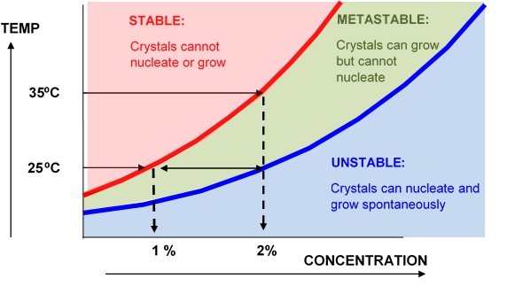
In the case above the solute has an equilibrium solubility of 1% at 25⁰C, and 2% at 35⁰C. A clean 2% solution cooled from 35⁰C to 25⁰C will still appear to be stable because there are no crystals to grow. However, the introduction of any nuclei would cause a rapid precipitation of half the material from solution. For this reason we do not normally use heat, ultrasound or high shear when measuring solubilities and we would usually ensure that there are nucleation sites present in the vessel.
2 Purity
High purity materials tend to have lower solubility than slightly impure materials, this is because impurities can get into the crystal lattice causing dislocations which change the chemical potential of the solid – in the same way that impurities lower the melting point. However, different types of impurity can have different effects, some can increase solubility but others can decrease solubility. For this reason if the source, grade or purity of the solute or solvent is changed in any way, the solubility and/or stability of the solute will need re-assessing.
3 Measurement Method
This is particularly important if the solute is a mixture – either by design or because it contains impurities. If we make a supersaturated mixture of solute and solvent and then measure how much is in solution we will be measuring the most soluble components of the mixture. However, if we take clean solvent and add solute to it until we see material out of solution then we would be measuring the least soluble component of the mixture.
4 Polymorphic Form
Polymorphism is all about minimising free energy.
Gibbs free energy equation:
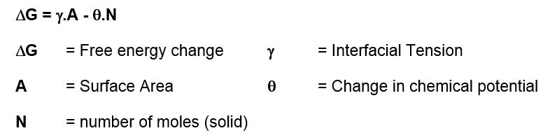
If ΔG is negative then crystals will always form as this is thermodynamically favoured. What is more difficult to derive is how long this might take, i.e. the kinetics. Almost all organic molecules are known to exist in many different polymorphic forms. By definition, the most stable polymorphic form of any material is the one with the lowest chemical potential. This means that the most stable polymorphic form must always be the least soluble. In practice what this means is that the supplied solute may often be in a more soluble polymorphic form, but it may change to a less soluble form when in solution via a process known as solvent mediated polymorphic phase transformation.
If we measure the wrong (less stable) polymorph we will always get too high a result for our solubility. For this reason we need to convert the solute to its most stable polymorphic form. This can usually be achieved by temperature cycling a saturated solution. The temperature cycling conditions required depend upon the solvent but usually a -10oC to +40oC daily cycle for a few days will suffice.
5 Particle Size
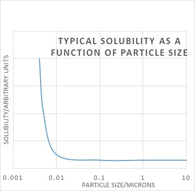 The same Gibbs free energy equation tells us that solubility is dependent on particle size, i.e. their surface area to volume ratio. It only really makes a difference when the particles are very small – 0.1 micron or less. Again we have the problem that measuring solubility of very small particles will give too high a result, and the solution will be unstable long-term because a process called Ostwald ripening will occur. The small crystals may well dissolve easily, but at some later stage large crystals will grow because they will have lower solubility and the solution will be supersaturated with respect to the larger crystals. For this reason we need to convert sub-micron solutes to larger crystal sizes via Ostwald ripening. This can also usually be achieved by temperature cycling a saturated solution as above.
6 Nucleation & Growth
Nucleation and growth are thermodynamically distinct processes, with nucleation being the initial formation of a crystallite of a critical size and then growth being the subsequent exponential increase in the crystal size.
Homogeneous vs Heterogeneous Nucleation
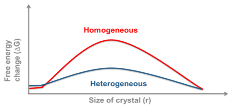
Again, this has practical implications for us. Homogeneous nucleation (in the absence of any nucleation sites) usually has a much higher free energy barrier than heterogeneous nucleation. The implication is that if we measure stability or solubility in clean laboratory glassware for instance, then we may be looking at a supersaturated solution. This may act like a true solution until the introduction of foreign nuclei results in sudden catastrophic crystallisation. On an industrial scale there will almost always be foreign bodies or rough surfaces to act as a scaffold for nucleation. For this reason we need to ensure that sufficient nucleation sites are available, this can be from scratching glassware or metal containers or by the intentional introduction of seed crystals.
7 Chemical Stability
Chemical stability refers to the propensity of the solute(s) or solvents to react or decompose in solution. The kinetics of the chemical reactions can be zero, first, or higher order. However, generally speaking, the observed responses for zero and first order reactions are indistinguishable for products that decompose relatively slowly.
Like all chemical reactions the decomposition rate decreases by a constant factor when the temperature is lowered. The relationship between temperature and the decomposition rate has been well characterized by the Arrhenius and related equations:
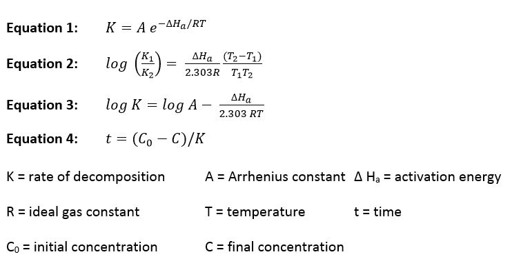
Given data on concentration vs. time data at two or more different temperatures we can calculate the rate constants for the reactions and the activation energy. This data then allows us to calculate the degree of decomposition at any other time/temperature as long as the following conditions are met:
(a) A zero- or first-order kinetics reaction takes place at each elevated temperature as well as at the real-life storage temperature. Theoretically, the Arrhenius equation does not apply when more than one kind of molecule is involved in reactions. However, if the decomposition rate and temperature are linearly related, the prediction of shelf life can still be approximated reasonably well.
(b) The same model is used to fit the decomposition patterns at each temperature, i.e. the temperature is not raised sufficiently high to enable new reaction paths.
We can therefore usually use short temperature stability studies at elevated temperatures to accurately predict long-term stability at lower temperatures.
References:
(1) Robert T Magari: “Assessing Shelf Life Using Real-Time and Accelerated Stability Tests”: BioPharm International Nov 1, 2003
(2) Geoffrey Anderson and MIlda Scott: “Determination of Product Shelf Life and Activation Energy for Five Drugs of Abuse”: Clin Chem 37/3, 398-402 (1991)
(3) Maria Nicoletti et al “Shelf-life of a 2.5% sodium hypochlorite solution as determined by Arrhenius equation”. Braz. Dent. Journal vol.20 no.1: 27-31 (2009)